Accumulation/Distribution Line: The Accumulation/Distribution Line is similar to the On Balance Volume (OBV), which sums the volume times +1/-1 based on whether the close is higher than the previous close. The Accumulation/Distribution indicator, however multiplies the volume by the close location value (CLV). The CLV is based on the movement of the issue within a single bar and can be +1, -1 or zero. The Accumulation/Distribution Line is interpreted by looking for a divergence in the direction of the indicator relative to price. If the Accumulation/Distribution Line is trending upward it indicates that the price may follow. Also, if the Accumulation/Distribution Line becomes flat while the price is still rising (or falling) then it signals an impending flattening of the price. The Accumulation/Distribution Line was developed by Marc Chaikin. The Accumulation/Distribution Line should not be confused with the Williams Price Accumulation/Distribution indicator.
Formula:
Accumulation Swing Index: The Accumulation Swing Index is a running total of the Swing Index. The Swing Index is calculated using only the two most recent bars, by summing it, the Accumulation Swing Index shows long-term trends. It will be positive in a long-term up trend, negative in a long-term down trend and it will hover around zero if the market is flat. The shape of the Accumulation Swing Index line closely matches the shape of the price line. It can be interpreted by comparing it to the price and looking for divergence or confirmation. The Accumulation Swing Index was developed by J. Welles Wilder and is described in his 1978 book New Concepts In Technical Trading Systems.
Formula:
Accumulate or Running Total: The Accumulate function calculates the running total of the input data. This is especially useful if the input data contains both positive and negative values so that the output will varry around zero.
Formula:
ADX - Average Directional Movement Index: The ADX is a Welles Wilder style moving average of the Directional Movement Index (DX). The values range from 0 to 100, but rarely get above 60. To interpret the ADX, consider a high number to be a strong trend, and a low number, a weak trend. See also +/-DI, DX and ADXR. The ADX was developed by J. Welles Wilder and is described in his 1978 book New Concepts In Technical Trading Systems.
Formula:
ADXR - Average Directional Movement Rating: The ADXR is equal to the current ADX plus the ADX from n bars ago divided by 2. In effect, it is the average of the two ADX values. The ADXR smoothes the ADX, and is therefore less responsive, however, the ADXR filters out excessive tops and bottoms. To interpret the ADXR, consider a high number to be a strong trend, and a low number, a weak trend. See also +/-DI, DX and ADX. The ADXR was developed by J. Welles Wilder and is described in his 1978 book New Concepts In Technical Trading Systems.
Formula:
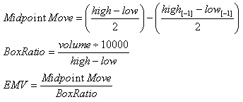
Ease of Movement: The EMV emphasizes days in which the stock is moving easily and minimizes the days in which the stock is finding it difficult to move. This indicator is used frequently with equivolume charts to identify market formations. A buy signal is generated when the EMV crosses above zero, a sell signal when it crosses below zero. When the EMV hovers around zero, then there are small price movements and/or high volume, which is to say, the price is not moving easily. The volume is divided by a volume increment (typically 10,000) to make the resultant numbers larger and easier to work with. The EMV is usually smoothed with a moving average. The Arms Ease of Movement indicator was developed by Richard W. Arms, Jr. See also Arms Index (TRIN).
Formula:
Aroon: The word aroon is Sanskrit for "dawn\'s early light". The Aroon indicator attempts to show when a new trend is dawning. The indicator consists of two lines (Up and Down) that measure how long it has been since the highest high/lowest low has occurred within an n period range. When the Aroon Up is staying between 70 and 100 then it indicates an upward trend. When the Aroon Down is staying between 70 and 100 then it indicates an downward trend. A strong upward trend is indicated when the Aroon Up is above 70 while the Aroon Down is below 30. Likewise, a strong downward trend is indicated when the Aroon Down is above 70 while the Aroon Up is below 30. Also look for crossovers. When the Aroon Down crosses above the Aroon Up, it indicates a weakening of the upward trend (and vice versa). The Aroon indicator was developed by Tushar S. Chande and first described in the September 1995 issue of Technical Analysis of Stocks & Commodities magazine.
Formula:
Aroon Oscillator: The Aroon Oscillator is calculated by subtracting the Aroon Down from the Aroon Up. The resultant number will oscillate between 100 and -100. The Aroon Oscillator will be high when the Aroon Up is high and the Aroon Down is low, indicating a strong upward trend. The Aroon Oscillator will be low when the Aroon Down is high and the Aroon Up is low, indicating a strong downward trend. When the Up and Down are approximately equal, the Aroon Oscillator will hover around zero, indicating a weak trend or consolidation. See the Aroon indicator for more information. The Aroon indicator was developed by Tushar S. Chande and first described in the September 1995 issue of Technical Analysis of Stocks & Commodities magazine.
Formula:
ATR - Average True Range: The ATR is a Welles Wilder style moving average of the True Range. The ATR is a measure of volatility. High ATR values indicate high volatility, and low values indicate low volatility, often seen when the price is flat. The ATR is a component of the Welles Wilder Directional Movement indicators (+/-DI, DX, ADX and ADXR). The ATR was developed by J. Welles Wilder and is described in his 1978 book New Concepts In Technical Trading Systems.
Formula:
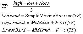
Bollinger Bands: Bollinger Bands consist of three lines. The middle band is a simple moving average (generally 20 periods) of the typical price (TP). The upper and lower bands are F standard deviations (generally 2) above and below the middle band. The bands widen and narrow when the volatility of the price is higher or lower, respectively. Bollinger Bands do not, in themselves, generate buy or sell signals: they are an indicator of overbought or oversold conditions. When the price is near the upper or lower band it indicates that a reversal may be imminent. The middle band becomes a support or resistance level. The upper and lower bands can also be interpreted as price targets. When the price bounces off of the lower band and crosses the middle band, then the upper band becomes the price target. See also Bollinger Width, Envelope, Price Channels and Projection Bands. Bollinger Bands were developed by John Bollinger.
Formula:
Bollinger Band Width: The Bollinger Band Width indicator is the distance between the upper and lower Bollinger Bands. It is a measure of volatility. The Band Width value is higher when volatility is high, and lower when volatility is low. High Band Width values indicate that the current trend may be about to end. Low Band Width values indicate that a new trend may be about to start. See also Bollinger Bands. Bollinger Bands were developed by John Bollinger.
Formula:
Commodity Channel Index (CCI): The CCI is designed to detect beginning and ending market trends. The range of 100 to -100 is the normal trading range. CCI values outside of this range indicate overbought or oversold conditions. You can also look for price divergence in the CCI. If the price is making new highs, and the CCI is not, then a price correction is likely. The Commodity Channel Index was developed by Donald Lambert and is described in his article in the October 1980 issue of Commodities magazine (now called Futures).
Formula:
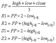
Chicago Floor Trading Pivotal Point: This function is used by floor traders on Chicago Mercantile Exchange to calculate short term support and resistence levels for commodities. It consists of two support an two resistance levels.
Formula:
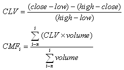
Chaikin Money Flow: The Chaikin Money Flow compares the total volume over the last n time periods to the total of volume times the Closing Location Value (CLV) over the last n time periods. The CLV calculates where the issue closes within its trading range. When the Chaikin Money Flow is above 0.25 it is a bullish signal, when it is below -0.25, it is a bearish signal. If the Chaikin Money Flow remains below zero while the price is rising, it indicates a probable reversal. The Chaikin Money Flow indicator was developed by Marc Chaikin.
Formula:
Chaikin Oscillator: The Chaikin Oscillator (AKA Chaikin A/D Oscillator) is essentially a momentum of the Accumulation/Distribution Line. It is calculated by subtracting a 10 period exponential moving average of the A/D Line from a 3 period exponential moving average of the A/D Line. When the Chaikin Oscillator crosses above zero, it indicates a buy signal, and when it crosses below zero it indicates a sell signal. Also look for price divergence to indicate bullish or bearish conditions. The Chaikin Oscillator was developed by Marc Chaikin.
Formula:
Chaikin Volatility: The Chaikin Volatility indicator is the rate of change of the trading range. The indicator defines volatility as a increasing of the difference between the high and low. A rapid increases in the Chaikin Volatility indicate that a bottom is approaching. A slow decrease in the Chaikin Volatility indicates that a top is approaching. The Chaikin Volatility indicator was developed by Marc Chaikin.
Formula:
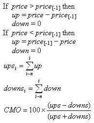
Chande Momentum Oscillator (CMO): The Chande Momentum Oscillator is a modified RSI. Where the RSI divides the upward movement by the net movement (up / (up + down)), the CMO divides the total movement by the net movement ((up - down) / (up + down)). There are several ways to interpret the CMO. Values over 50 indicate overbought conditions, while values under -50 indicate oversold conditions. High CMO values indicate strong trends. When the CMO crosses above a moving average of the CMO, it is a buy signal, crossing down is a sell signal. The Chande Momentum Oscillator was developed by Tushar S. Chande and is described in the 1994 book The New Technical Trader by Tushar S. Chande and Stanley Kroll.
Formula:
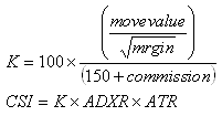
Commodity Selection Index (CSI): The Commodity Selection Index is a composite indicator calculated by multiplying the ADXR (Average Directional Movement Rating) and the ATR (Average True Range) by a constant that incorporates the move value, commission and margin. The CSI selects commodities that are suitable for short term trading (those with high CSI values). The Commodity Selection Index was developed by J. Welles Wilder and is described in his 1978 book New Concepts In Technical Trading Systems.
Formula:
DEMA: The DEMA is a smoothing indicator with less lag than a straight exponential moving average. DEMA is an acronym for Double Exponential Moving Average, but the calculation is more complex than just a moving average of a moving average. The DEMA was developed by Patrick Mulloy and is described in his article in the February, 1994 issue of Technical Analysis of Stocks & Commodities magazine. See also Exponential Moving Average, TEMA and T3.
Formula:
Demand Index: The Demand Index is a market strength indicator based on price and volume that calculates a ratio buying pressure to selling pressure. It can be a leading indicator of price moves. The Demand Index can be interpreted by looking for divergence with price to indicate impending price moves. Peaks in the Demand Index signal a coming peak in price. When the Demand Index hovers around zero, it indicates weak price moves. The Demand Index was developed by James Sibbet.
Formula:
De-trended Price: The De-trended Price first calculates a regression line for a time series, then subtracts the slope of the line from the price. By removing the trend from the time series, the result is a series of detrended prices. It has the effect of flattening out the trend to make oscillations more visible.
Formula:
Detrended Price Oscillator (DPO): The Detrended Price Oscillator removes the trend in prices by subtracting a moving average of the price from the price. The Detrended Price shows cycles and overbought/oversold conditions. Note that the calculation shifts the results (shift = term / 2 + 1) periods, so the last shift periods will be zero. The size property of the output array is set accordingly, and the last shift periods will not be graphed.
Formula:
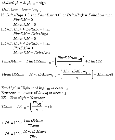
Directional Movement Index (+DI and -DI): The +DI is the percentage of the true range that is up. The -DI is the percentage of the true range that is down. A buy signal is generated when the +DI crosses up over the -DI. A sell signal is generated when the -DI crosses up over the +DI. You should wait to enter a trade until the extreme point is reached. That is, you should wait to enter a long trade until the price reaches the high of the bar on which the +DI crossed over the -DI, and wait to enter a short trade until the price reaches the low of the bar on which the -DI crossed over the +DI. See also DX, ADX and ADXR. The DI was developed by J. Welles Wilder and is described in his 1978 book New Concepts In Technical Trading Systems.
Formula:
Directional Movement Index (DX): The DX is usually smoothed with a moving average (i.e. the ADX). The values range from 0 to 100, but rarely get above 60. To interpret the DX, consider a high number to be a strong trend, and a low number, a weak trend. See also +/-DI, ADX and ADXR. The DX was developed by J. Welles Wilder and is described in his 1978 book New Concepts In Technical Trading Systems.
Formula:
Down Average: The Down Average is a Welles Wilder style moving average of the decreases between consecutive prices. Used in the calculation of the RSI.
Formula:
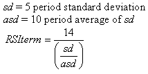
Dynamic Momentum Index (DMI): The Dynamic Momentum Index is a variable term RSI. The RSI term varies from 3 to 30. The variable time period makes the RSI more responsive to short-term moves. The more volatile the price is, the shorter the time period is. It is interpreted in the same way as the RSI, but provides signals earlier. See also RSI. The Dynamic Momentum Index was developed by Tushar S. Chande and Stanley Kroll and is described in their 1994 book The New Technical Trader.
Formula:
Envelope Percent: The Envelope Percent function creates plus and minus bands arround series of numbers, based on a percentage of the series. A common use is creating support/resistence bands around the close. See also Envelolpe, Bollinger Bands, Price Channels and Projection Bands.
Formula:
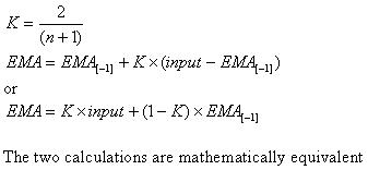
Exponential Moving Average: The Exponential Moving Average is a staple of technical analysis and is used in countless technical indicators. In a Simple Moving Average, each value in the time period carries equal weight, and values outside of the time period are not included in the average. However, the Exponential Moving Average is a cumulative calculation, including all data. Past values have a diminishing contribution to the average, while more recent values have a greater contribution. This method allows the moving average to be more responsive to changes in the data. See also Least Squares MA, Simple MA, Triangular MA, Weighted MA, Welles MA, Variable MA, Volume Adjusted MA, Zero Lag Exponential MA, DEMA, TEMA and T3.
Formula:
Herrick Payoff Index: The Herrick Payoff Index measures the money flowing in and out of a futures contract based on the trading range, volume and open interest. The HPI is interpreted by looking for divergence with the price. The Herrick Payoff Index was developed by John Herrick.
Formula:
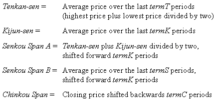
Ichimoku Kinko Hyo: Ichimoku Kinko Hyo is Japanese for "one glance cloud chart." It consists of five lines called Tenkan-sen, Kijun-sen (sen is Japanese for line), Senkou Span A, Senkou Span B and Chinkou Span. The calculation uses four different time periods which we call termT, termK, termS and termC. The Ichimoku Kinko Hyo is graphed over the closing price line. The space between the Senkou spans is called the Cloud, and is usually graphed in a hatched pattern. The Senkou Spans are support and resistance lines. When the price is in the Cloud, the market is non-trending. When the price is above the Cloud, the higher Span is the first support level and the lower Span is the second support level. When the price is below the Cloud, the lower Span is the first resistance level and the higher Span is the second resistance level. Kijun-sen and Tenkan-sen are trend indicators. When the price is above the Kijun-sen, prices will likely continue to go up, when the price is below the Kijun-sen, prices will likely continue to go down. The direction of the Tenkan-sen indicates the direction of the trend. If the Tenkan-sen is flat, the market is in a non-trending channel. A buy signal is generated when the Chinkou Span crosses over the price, or when the Tenkan-sen crosses over the Kijun-sen. A sell signal is generated when the Chinkou Span crosses under the price, or when the Tenkan-sen crosses under the Kijun-sen. Look for confirmation when both crosses occur. The Ichimoku Kinko Hyo was developed by Goichi Hosoda before WWII, and published in 1969.
Formula:
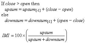
Intraday Momentum Index (IMI): The Intraday Momentum Index is similar to the RSI, but uses the movement between the open and close whereas the RSI uses the movement between the close and the previous close. IMI values over 70 indicate an overbought condition, and values under 30 indicate oversold. The Intraday Momentum Index was developed by Tushar S. Chande and Stanley Kroll and is described in their 1994 book The New Technical Trader.
Formula:
Inertia: The Inertia indicator is the Relative Volatility Index (RVI) smoothed with a Least Squares Moving Average. Like the RVI, the Inertia ranges from 0 to 100. Inertia signals long-term trends. Positive Inertia is indicated by values above 50, while values below 50 indicate negative inertia (slowing). The Inertia indicator was developed by Donald Dorsey and was introduced his article in September, 1995 issue of Technical Analysis of Stocks & Commodities magazine.
Formula:
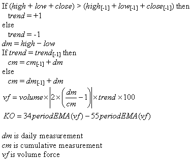
Klinger Oscillator (KO): The Klinger Oscillator uses a combination of high-low trading range, volume and accumulation/distribution to find trading tops and bottoms. The KO is used with a signal line which is a 13 period Exponential Moving Average of the KO. To interpret the KO, look for divergence with the price to signal the coming end of a trend, or to indicate that rising/falling prices are not forming a new trend. A buy signal is generated when the KO rises from below zero to cross above the trigger line. A sell signal is generated when the KO falls from its high and crosses below the trigger line. The Klinger Oscillator is also known as the Klinger Volume Oscillator or KVO. The Klinger Oscillator was developed by Stephen J. Klinger and was first presented in his article in the Winter 1994/Spring 1995 issue of MTA Journal.
Formula:
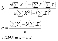
Least Squares Moving Average: The Least Squares Moving Average first calculates a least squares regression line over the preceding time periods, then projects it forward to the current period. In essence, it calculates what the value would be if the regression line continued. The Least Squares Moving Average is also known as an Endpoint Moving Average, a Time Series Moving Average or a Time Series Forecast. See also Exponential MA, Simple MA, Triangular MA, Weighted MA, Welles MA, Variable MA, Volume Adjusted MA, Zero Lag Exponential MA, DEMA, TEMA and T3.
Formula:
Mass Index: The Mass Index is a moving sum of a 9 period Exponential Moving Average of the trading range (high minus low) divided by the double smoothed moving average of the range. The Mass Index is intended to identify trend reversals. Higher Mass Index values are created by widening trading ranges, which indicate a trend reversal. The MASS Index was developed by Donald Dorsey and was presented in his article in the June, 1992 issue of Technical Analysis of Stocks & Commodities magazine.
Formula:
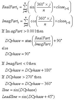
MESA Sinewave: The Mesa Sine Wave calculates two sine curves. When the two curves resemble a sine wave, the market is in a cycle, otherwise the market is trending. Signals are generated only when the market is in a cycle. A buy signal is generated when the Sine crosses up over the Lead Sine, and a sell signal when the Sine crosses down below the Lead Sine. The Mesa Sine Wave was developed by John Elhers and was introduced in his article in the November, 1996 issue of Technical Analysis of Stocks & Commodities magazine.
Formula:
Market Facilitation Index (MFI): Market Facilitation Index (MFI) is the trading range divided by the volume. The MFI measures the price movement per unit of volume. To interpret the MFI, compare it to the volume. When the MFI is high and volume is low, it signals a fake trend which will soon reverse. When the MFI is low and volume is high, it signals a new trend in either direction is about to occur. When the MFI is low and volume is also low, it signals a fading market and an impending trend reversal. When the MFI is high and volume is also high, it signals a strong trend. The Market Facilitation Index was developed by Dr. Bill Williams and is described in his 1995 book, Trading Chaos.
Formula:
Momentum: The Momentum is a measurement of the acceleration and deceleration of prices. It indicates if prices are increasing at an increasing rate or decreasing at a decreasing rate. The Momentum function can be applied to the price, or to any other data series.
Formula:
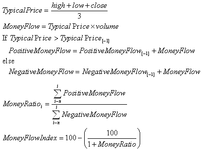
Money Flow Index: The Money Flow Index calculates the ratio of money flowing into and out of a security. To interpret the Money Flow Index, look for divergence with price to signal reversals. Money Flow Index values range from 0 to 100. Values above 80/below 20 indicate market tops/bottoms.
Formula:
Moving Average: The Moving Average function calculates a moving average using one of eight methods: Exponential, Least Squares, Simple, Triangular, Variable, Weighted, Welles Wilder style, or Zero Lag Exponential. The purpose of the function is to make it easy to change the calculation method by just changing one parameter.
Formula:
Moving Average Convergence/Divergence (MACD): The Moving Average Convergence Divergence (MACD) is the difference between two Exponential Moving Averages. The Signal line is an Exponential Moving Average of the MACD. The MACD signals trend changes and indicates the start of new trend direction. High values indicate overbought conditions, low values indicate oversold conditions. Divergence with the price indicates an end to the current trend, especially if the MACD is at extreme high or low values. When the MACD line crosses above the signal line a buy signal is generated. When the MACD crosses below the signal line a sell signal is generated. To confirm the signal, the MACD should be above zero for a buy, and below zero for a sell. The time periods for the MACD are often given as 26 and 12. However the function actually uses exponential constants of 0.075 and 0.15, which are closer to 25.6667 and 12.3333 periods. To create a similar indicator with time periods other than those built into the MACD, use the Price Oscillator function. The MACD was developed by Gerald Appel.
Formula:
Moving Average Envelope: The MA Envelope function creates high and low bands around a moving average.
Formula:
Moving Averages of the High and Low: The MA High Low function creates moving averages of the high and the low.
Formula:
Moving Dispersion: The Moving Dispersion calculates the absolute change between values over a given time period.
Formula:
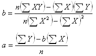
Moving Regression Line: The Moving Regression Line function fills two output arrays with the slope and constant of a least squares regression line of the input data series over the given time period. This function is used in the calculation of several indicators. It can be used to calculate the slope of the price or any indicator.
Formula:
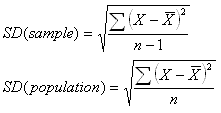
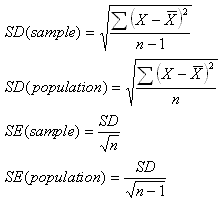
Moving Standard Deviation: The Moving Standard Deviation function fills the output Array with the standard deviation of the last n values of the input Array. This function is used in the calculation of several indicators. It can take price or the output of any indicator as its input. Standard Deviation is often used as a measure of volatility.
Formula:
Moving Standard Error: The Moving Standard Error function fills the output Array with the standard error of the last n values of the input Array. This function is used in the calculation of several indicators. It can take price or the output of any indicator as its input.
Formula:
Moving Summation: The moving summation is the sum of the last n values. It is a Simple Moving Average without dividing the sum by n. The moving sum is used in the calculation of many indicators. It can also be used to modify any existing indicator.
Formula:
Net Momentum Oscillator (NMO): The Net Momentum Oscillator (NMO) is a variation on the RSI. Whereas the RSI based on the ratio of up periods to down periods, the NMO is the ratio of the momentum (up - down) to the absolute momentum (up + down) . The NMO is able to show overbought and oversold levels (greater than +50, less than -50) better than the RSI. The Net Momentum Oscillator was developed by Tushar Chande and Stanley Kroll and was introduced in their article in the May, 1993 issue of Technical Analysis of Stocks & Commodities magazine.
Formula:
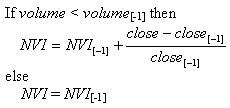
Negative Volume Index (NVI): Negative Volume Index (NVI) attempts to identify bull markets by showing what the smart investors are doing. It is based on the assumption smart investors dominate trading on light volume days and uninformed investors dominates trading on active days. The NVI changes on days when the volume is down and stays flat on up volume days. Look for the NVI to rise above its one year moving average to signal a bull market. Also see the Positive Volume Index. The Negative and Positive Volume Index were developed by Norman Fosback and are described in his 1976 book, Stock Market Logic.
Formula:
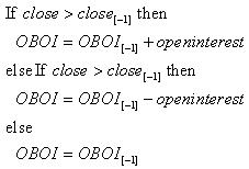
On Balance Open Interest (OBOI): The On Balance Open Interest (OBOI) is a total of the up and down open interest. The calculation is based on the On Balance Volume (OBV). When the close is higher than the previous close, the open interest is added to the running total, and when the close is lower than the previous close, the open interest is subtracted from the running total. This version of the OBOI is a moving total, not a cumulative total. That is, only the values from the past n days are totaled.
Formula:
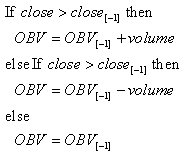
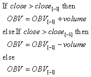
On Balance Volume (OBV): The On Balance Volume (OBV) is a cumulative total of the up and down volume. When the close is higher than the previous close, the volume is added to the running total, and when the close is lower than the previous close, the volume is subtracted from the running total. To interpret the OBV, look for the OBV to move with the price or precede price moves. If the price moves before the OBV, then it is a non-confirmed move. A series of rising peaks, or falling troughs, in the OBV indicates a strong trend. If the OBV is flat, then the market is not trending. The On Balance Volume was developed by Joseph Granville and is described in his 1963 book, New Strategy of Daily Stock Market Timing for Maximum Profit.
Formula:
On Balance Volume, Expanded System: The On Balance Volume, Expanded System calculates OBV and identifies the breakouts and field trends as described in Joseph Granville\'s 1963 book New Strategy of Daily Stock Market Timing for Maximum Profit. The breakout Array is filled with the following codes: 1 = up, -1 = down, 0 = no breakout on this bar. The fieldtrend Array is filled with the following codes: 1 = rising, -1 = falling, 0 = doubtfull. Also see On Balance Volume and On Balance Volume, Moving.
Formula:
On Balance Volume, Moving: This version of the On Balance Volume (OBV) is a moving total, not a cumulative total. That is, only the values from the past n days are totaled, as opposed to totaling all days from the beginning of the data series. See On Balance Volume for more information. Also see On Balance Volume, Expanded System. The Oscillator function calculates the difference between two data series. It is a generic function that can take any price or indicator data as input. It is used in the calculation of many indicators.
Formula:
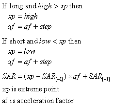
Parabolic SAR: The Parabolic SAR calculates a trailing stop. Simply exit when the price crosses the SAR. The SAR assumes that you are always in the market, and calculates the Stop And Reverse point when you would close a long position and open a short position or vice versa. The Parabolic SAR was developed by J. Welles Wilder and is described in his 1978 book, New Concepts In Technical Trading Systems.
Formula:
Performance Indicator: The Performance indicator displays the percentage difference between the price today and the price at the start of the data series. It is also known as a normalized price. It can be useful for comparing the performance of two securities or a security and an index.
Formula:
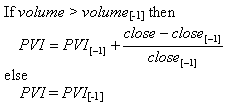
Positive Volume Index (PVI): The Positive Volume Index (PVI) attempts to identify bull markets. The PVI shows what the uninformed investors are doing, while the Negative Volume Index shows what the smart investors are doing. It is based on the assumption smart investors dominate trading on light volume days and uninformed investors dominates trading on active days. The PVI changes on days when the volume is up and stays flat on down volume days. Also see the Negative Volume Index. The Positive and Negative Volume Index were developed by Norman Fosback and are described in his 1976 book, Stock Market Logic.
Formula:
Percentage Volume Oscillator (PVO): The Percentage Volume Oscillator (PVO) is the percentage difference between two moving averages of volume. The PVO has a maximum of 100, but no minimum value. PVO crosses over zero when the fast Exponential Moving Average (EMA) is greater than the slow EMA indicating that volume is above average. The PVO crosses below zero when the fast EMA is less than the slow EMA indicating that volume is below average. The direction of the PVO curve indicates rising or falling volume levels. Look for strong volume (rising PVO) to confirm price trends. A moving average of the PVO can be used as a signal line to indicate longer term movements and to look for crossovers.
Formula:
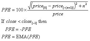
Polarized Fractal Efficiency (PFE): The Polarized Fractal Efficiency indicator uses fractal geometry to determine how efficiently the price is moving. When the PFE is zigzagging around zero, then the price is congested and not trending. When the PFE is smooth and above/below zero, then the price is in an up/down trend. The higher/lower the PFE value, the stronger the trend is. The Polarized Fractal Efficiency indicator was developed by Hans Hannula and was introduced in the January, 1994 issue of Technical Analysis of Stocks & Commodities magazine.
Formula:
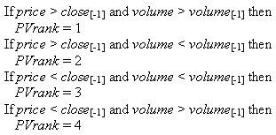
Price Volume Rank: The Price Volume Rank was developed as a simple indicator that could be calculated even without a computer. The basic interpretation is to buy when the PV Rank is below 2.5 and sell when it is above 2.5. The Price Volume Rank was developed by Anthony J. Macek and is described in his article in the June, 19994 issue of Technical Analysis of Stocks & Commodities magazine.
Formula:
Price and Volume Trend (PVT): The Price Volume Trend (PVT) is similar to the On Balance Volume (OBV). The OBV is a cumulative total of volume times +1/-1 based on whether the close is greater or less than the previous close. However, the PVT is a cumulative total of volume times the percentage change of the close from the previous close. So, it adds more of the volume to the total when the price makes greater moves. The PVT is interpreted in the same ways as the OBV. See also On Balance Volume.
Formula:
Price Channels: The Price Channels indicator creates a high band of the highest high over the last n periods and a low band of the lowest low over the last n periods. The bands are support and resistance levels. See also Bollinger Bands, Envelope and Projection Bands.
Formula:
Price Oscillator: The Price Oscillator shows the difference between two moving averages. It is basically a MACD, but the Price Oscillator can use any time periods. A buy signal is generate when the Price Oscillator rises above zero, and a sell signal when the it falls below zero. See also Price Oscillator Percent, MACD.
Formula:
Price Oscillator, Percent: The Price Oscillator Percent shows the percentage difference between two moving averages. A buy signal is generate when the Price Oscillator Percent rises above zero, and a sell signal when the it falls below zero. See also Price Oscillator.
Formula:
Projection Bands: Projection Bands are calculated by finding the highest high and lowest low over the last n periods and plotting them parallel to a regression line of the high/low. The Projection Bands are support and resistance levels. When the price reaches the upper band, it signals a price top and probable reversal. Likewise, when the price reaches the bottom band, it signals a bottom. The price will never actually break above or below the bands (unlike Bollinger Bands). See also Projection Bandwidth and Projection Oscillator. For other types of bands, see Bollinger Bands, Envelope and Price Channels. Projection Bands were developed by Mel Widner, Ph.D and were originally introduced in his article in the July, 1995 issue of Technical Analysis of Stocks & Commodities magazine.
Formula:
Projection Bandwidth: Projection Bandwidth is based on the Projection Bands indicator. It is the ratio of the width of the bands to the midpoint. A low number indicates that the bands are narrowing, a high number means that the bands are widening. The band width is a measure of volatility. Narrow bands mean a narrow trading range and low volatility: wide bands, wide range, high volatility. See also Projection Bands and Projection Oscillator. Projection Bands were developed by Mel Widner, Ph.D and were originally introduced in his article in the July, 1995 issue of Technical Analysis of Stocks & Commodities magazine.
Formula:
Projection Oscillator: The Projection Oscillator is based on the Projection Bands indicator. The Oscillator calculates where the close lies within the band as a percentage. Therefore, an Oscillator value of 50 would mean that the close is in the middle of the band. A value of 100 would mean that the close is equal to the top band, and zero means that it is equal to the low band. The calculation is similar to a Stochastic which uses the raw highest high and lowest low value, whereas the Projection Oscillator adds the regression line component, making it more sensitive. The Projection Oscillator can be interpreted several ways. Look for divergence with price to indicate a trend reversal. Extreme values (over 80 or under 20) indicate overbought/oversold levels. A moving average of the oscillator can be used as a trigger line. A buy/sell signal is generated when the Projection Oscillator to cross above/below the trigger line. The signal is stronger if it happens above 70 or below 30. See also Projection Bands and Projection Bandwidth. Projection Bands were developed by Mel Widner, Ph.D and were originally introduced in his article in the July, 1995 issue of Technical Analysis of Stocks & Commodities magazine.
Formula:
Qstick: The Qstick indicator is an exponential moving average of the difference between the open and close. The "stick" in the name comes from candlestick charting. The body of a candlestick is from the open to the close. A white candlestick is an up and a black candlestick is a down day. Positive Qstick values indicate a majority of up days: negative values, a majority of down days. To interpret the Qstick, look for a buy signal when it crosses above zero, and a sell signal when it crosses below zero. Also look for a buy signal when the Qstick is very low and turns up, and a sell signal when it is very high and turns down. A moving average of the Qstick can be used as a trigger line (look for the Qstick to cross the trigger). You can also look for divergence between the Qstick and price to indicate the end of a trend or as a non-confirmation of a price move. The Qstick indicator was developed by Tushar S. Chande and Stanley Kroll and is described in their 1994 book The New Technical Trader.
Formula:
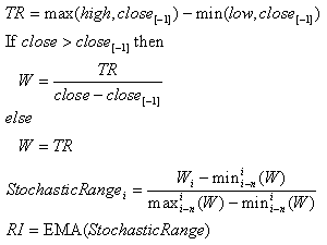
Range Indicator: The Range indicator compares the intraday range (high - low) to the inter-day (close - previous close) range. When the intraday range is greater than the inter-day range, the Range Indicator will be a high value. This signals an end to the current trend. When the Range Indicator is at a low level, a new trend is about to start. The Range Indicator was developed by Jack Weinberg and was introduced in his article in the June, 1995 issue of Technical Analysis of Stocks & Commodities magazine.
Formula:
Rate of Change: The Rate of Change function measures rate of change relative to previous periods. The function is used to determine how rapidly the data is changing. The factor is usually 100, and is used merely to make the numbers easier to interpret or graph. The function can be used to measure the Rate of Change of any data series, such as price or another indicator. When used with the price, it is referred to as the Price Rate Of Change, or PROC.
Formula:
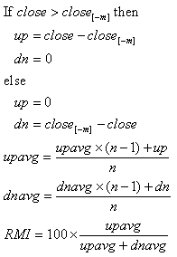
Relative Momentum Index (RMI): The Relative Momentum Index (RMI) is a variation on the Relative Strength Index (RSI). To determine up and down days, the RSI uses the close compared to the previous close. The RMI uses the close compared to the close n days ago. An RMI with a time period of 1 is equal to the RSI. The RMI ranges from 0 to 100. Loke the RSI, The RMI is interpreted as an overbought/oversold indicator when the value is over 70/below 30. You can also look for divergence with price. If the price is making new highs/lows, and the RMI is not, it indicates a reversal. See also Relative Strength Index. The Relative Momentum Index was developed by Roger Altman and was introduced in his article in the February, 1993 issue of Technical Analysis of Stocks & Commodities magazine.
Formula:
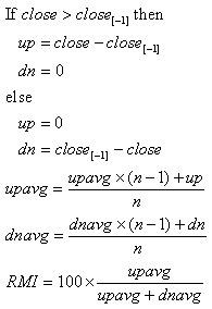
Relative Strength Index (RSI): The Relative Strength Index (RSI) calculates a ratio of the recent upward price movements to the absolute price movement. The RSI ranges from 0 to 100. The RSI is interpreted as an overbought/oversold indicator when the value is over 70/below 30. You can also look for divergence with price. If the price is making new highs/lows, and the RSI is not, it indicates a reversal. The Relative Strength Index (RSI) was developed by J. Welles Wilder and was first introduced in his article in the June, 1978 issue of Commodities magazine, now known as Futures magazine, and is detailed in his book New Concepts In Technical Trading Systems.
Formula:
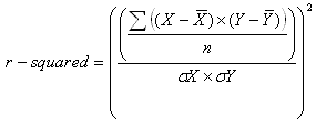
r-squared: The r-squared indicator calculates how well the price approximates a linear regression line. The indicator gets its name from the calculation, which is, the square of the correlation coefficient (referred to in mathematics by the Greek letter rho, or r). The range of the r-squared is from zero to one. High r-squared values indicate a strong correlation, and an indication of a trend. An r-squared value above the critical value listed below indicates a positive correlation between the price and the linear regression line with 95% confidence. n r-squared 5 .77 10 .40 14 .27 20 .20 25 .16 30 .13 50 .08 60 .06 120 .03
Formula:
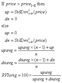
Relative Volatility Index (RVI): The Relative Volatility Index (RVI) is based on the Relative Strength Index (RSI). Whereas the RSI uses the average price change, the RVI uses a 9 period standard deviation of the price.
Formula:
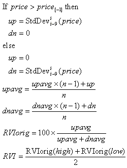
Relative Volatility Index (RVI) - Original Calculation: The RVI indicator is a revision of the original RVI. The original version of the RVI is calculated using the closing price. The revised version is calculated by taking the average of the original RVI of the high and the original RVI of the low. See Relative Volatility Index - Original Calculation for the original version. The RVI is a volatility indicator. It was developed as a compliment to and a confirmation of momentum based indicators. When used to confirm other signals, only buy when the RVI is over 50 and only sell when the RVI is under 50. If a signal is ignored, buy when the RVI is over 60 and sell when the RVI is under 40. Exit a long position if the RVI drops below 40 and exit a short position when the RVI rises above 60. Also see the RVI Original. The Relative Volatility Index was developed by Donald Dorsey and was originally introduced in his article in the June, 1993 issue of Technical Analysis of Stocks & Commodities magazine, and later revised in his article in the September, 1995 issue of the same magazine.
Formula:
Random Walk Index (RWI): The Random Walk Index (RWI) is used to determine if an issue is trending or in a random trading range by comparing it to a straight line. The more random the price movement, the more the RWI fluctuates. The short-term (2 to 7 periods) RWI is an overbought/oversold indicator, while the long-term (8 to 64 periods) RWI is a trend indicator. An issue is trending higher if the RWI of the highs is greater than 1, while a downtrend is indicated if the RWI of the lows is greater than 1. A buy signal is generated when the long-term RWI of the highs is greater than 1 and the short-term RWI of the lows rises above 1. A sell signal is generated when the long-term RWI of the lows is greater than 1 and the short-term RWI of the highs rises above 1. The Random Walk Index was developed by Michael Poulos and is described in his article in the February, 1991 issue of Technical Analysis of Stocks & Commodities magazine.
Formula:
Simple Moving Average: Moving Averages are used to smooth the data in an array to help eliminate noise and identify trends. The Simple Moving Average is literally the simplest form of a moving average. Each output value is the average of the previous n values. In a Simple Moving Average, each value in the time period carries equal weight, and values outside of the time period are not included in the average. This makes it less responsive to recent changes in the data, which can be useful for filtering out those changes. See also Exponential MA, Least Squares MA, Triangular MA, Weighted MA, Welles MA, Variable MA, Volume Adjusted MA, Zero Lag Exponential MA, DEMA, TEMA and T3.
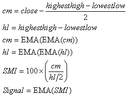
Stochastic Momentum Index (SMI): The Stochastic Momentum Index (SMI) is based on the Stochastic Oscillator. The difference is that the Stochastic Oscillator calculates where the close is relative to the high/low range, while the SMI calculates where the close is relative to the midpoint of the high/low range. The values of the SMI range from +100 to -100. When the close is greater than the midpoint, the SMI is above zero, when the close is less than than the midpoint, the SMI is below zero. The SMI is interpreted the same way as the Stochastic Oscillator. Extreme high/low SMI values indicate overbought/oversold conditions. A buy signal is generated when the SMI rises above -50, or when it crosses above the signal line. A sell signal is generated when the SMI falls below +50, or when it crosses below the signal line. Also look for divergence with the price to signal the end of a trend or indicate a false trend. The Stochastic Momentum Index was developed by William Blau and was introduced in his article in the January, 1993 issue of Technical Analysis of Stocks & Commodities magazine.
Formula:
Standard Error Bands: Standard Error Bands are a type of envelope. They look similar to Bollinger Bands, however the calculation and interpretation is different. The middle band is a Least Squares Moving Average. The high band is the middle band plus a factor times the n period standard error. The low band is the middle band minus a factor times the n period standard error. When the bands are close together, it means that there is a low standard error, which means that the price is in a trend. When the bands are farther apart, then the price is not trending. When the price is in a trend and the bands are close together, look for the bands to widen to signal the end of the trend. Standard Error Bands were developed by Jon Anderson.
Formula:
General Stochastic Calculation: This is a general form of the Lane Stochastic Oscillator calculation that works on any Array, instead of Bars. This is very usefull for building composite indicators. The general Stochastic theory still applies, that is, that as prices decrease, they tend to accumulate near the extreme lows, and when rising, they tend to accumulate near the extreme highs.
Formula:
Stochastic Oscillator: The Stochastic Oscillator measures where the close is in relation to the recent trading range. The values range from zero to 100. %D values over 75 indicate an overbought condition; values under 25 indicate an oversold condition. When the Fast %D crosses above the Slow %D, it is a buy signal; when it crosses below, it is a sell signal. The Raw %K is generally considered too erratic to use for crossover signals. Also see the General Stochastic Calculation. The Stochastic Indicator was developed by George C. Lane. Terminology:
Fast Stochastic Refers to both %K and %D where %K is un-smoothed
Slow Stochastic Refers to both %K and %D where %K is smoothed
Raw %K Un-smoothed %K
Fast %K Un-smoothed %K
Slow %K Smoothed %K
Fast %D Moving average of an un-smoothed %K
Slow %D Moving average of a smoothed %K, in effect: a double smoothed %K.
Always refers to a smoothed %K (whether or not the %K itself is smoothed).
Formula:
Stochastic RSI: Stochastic RSI (StochRSI) is an indicator of an indicator. It calculates the Relative Strength Indicator (RSI) relative to its range in order to increase the sensitivity of the standard RSI. The values of the StochRSI are from zero to one. The Stochastic RSI can be interpreted several ways. Overbought/oversold conditions are indicated when the StochRSI crosses above .20 / below .80. A buy signal is generated when the StochRSI moves from oversold to above the midpoint (.50). A sell signal is generated when the StochRSI moves from overbought to below the midpoint. Also look for divergence with the price to indicate the end of a trend. See also Stochastic, Stochastic Oscillator and RSI. The Stochastic RSI was developed by Tushar S. Chande and Stanley Kroll and is described in their 1994 book, The New Technical Trader.
Formula:
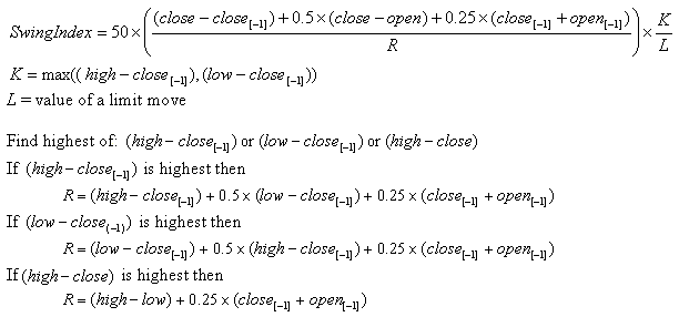
Swing Index: The Swing Index attempts to determine the real price. The numbers range from -100 to +100. It is difficult to interpret in its raw form, and is usually summed to form the Accumulation Swing Index. It is important to use the correct limit move for the commodity you are analyzing (e.g. $3.00 for T-Bonds, $0.04 for Heating Oil, etc). For a stock, limit move should be a large number, such as $10,000. The Swing Index was developed by J. Welles Wilder and is described in his 1978 book New Concepts In Technical Trading Systems.
Formula:
T3: The T3 is a type of moving average, or smoothing function. It is based on the DEMA. The T3 takes the DEMA calculation and adds a vfactor which is between zero and 1. The resultant function is called the GD, or Generalized DEMA. A GD with vfactorof 1 is the same as the DEMA. A GD with a vfactor of zero is the same as an Exponential Moving Average. The T3 typically uses a vfactor of 0.7. The T3 triple-smoothes the data series by calling the GD three times. You can pass any value for tcount to the T3 function. For instance, a tcountof 4 would be quadruple-smoothed, in effect a T4. A tcount of 1 would be a single-smoothed GD. Any data series can be smoothed with the T3, including price or the output of another indicator. See also Exponential Moving Average, DEMA and TEMA. The T3 was developed by Tim Tillson and was described in his January, 1998 article in Technical Analysis of Stocks & Commodities magazine.
Formula:
TEMA: The TEMA is a smoothing indicator with less lag than a straight exponential moving average. TEMA is an acronym for Triple Exponential Moving Average, but the calculation is more complex than that. The TEMA was developed by Patrick Mulloy and is described in his article in the January, 1994 issue of Technical Analysis of Stocks & Commodities magazine. See also Exponential Moving Average, DEMA and T3.
Formula:
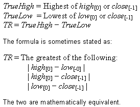
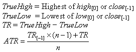
True Range (TR): The True Range function is used in the calculation of many indicators, most notably, the Welles Wilder DX. It is a base calculation that is used to determine the normal trading range of a stock or commodity.
Formula:
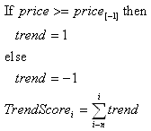
Trend Score: The Trend Score is a simple indicator that attempts to show when price is trending by looking at up and down days. The trend is equal to one when the price is greater than or equal to the previous price, and as a negative one when the price is less than the previous price. The Trend Score is the moving summation of those ones and negative ones over the past n periods.
Formula:
Triangular Moving Average: The Triangular Moving Average is a form of Weighted Moving Average wherein the weights are assigned in a triangular pattern. For example, the weights for a 7 period Triangular Moving Average would be 1, 2, 3, 4, 3, 2, 1. This gives more weight to the middle of the time series and less weight to the oldest and newest data. The Triangular Moving Average is mathematically equivalent to a Simple Moving Average of a Simple Moving Average. See also Exponential MA, Least Squares MA, Simple MA, Weighted MA, Welles MA, Variable MA, Volume Adjusted MA, Zero Lag Exponential MA, DEMA, TEMA and T3.
Formula:
TRIX: The TRIX indicator calculates the rate of change of a triple exponential moving average. The values oscillate around zero. Buy/sell signals are generated when the TRIX crosses above/below zero. A (typically) 9 period exponential moving average of the TRIX can be used as a signal line. A buy/sell signals are generated when the TRIX crosses above/below the signal line and is also above/below zero. The TRIX was developed by Jack K. Hutson, publisher of Technical Analysis of Stocks & Commodities magazine, and was introduced in Volume 1, Number 5 of that magazine.
Formula:
True Strength Index (TSI): The True Strength Index (TSI) is a variation of the Relative Strength Index (RSI). The TSI uses a double smoothed exponential moving average of price momentum to eliminate choppy price changes and spot trend changes. This indicator has a little or no time lag. The True Strength Index was developed by William Blau and is described in his 1995 book Momentum, Direction, and Divergence.
Formula:
Typical Price: The Typical Price is the average of the high + low + close of a bar. It is used in the calculation of several indicators. It can be used to smooth an indicator that normally takes just the closing price as input. See also Average Price, Median Price and Weighted Close.
Formula:
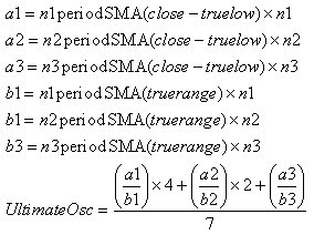
Ultimate Oscillator: The Ultimate Oscillator is the weighted sum of three oscillators of different time periods. The typical time periods are 7, 14 and 28. The values of the Ultimate Oscillator range from zero to 100. Values over 70 indicate overbought conditions, and values under 30 indicate oversold conditions. Also look for agreement/divergence with the price to confirm a trend or signal the end of a trend. The Ultimate Oscillator was developed by Larry Williams and was introduced in his article in the April, 1985 issue of Technical Analysis of Stocks & Commodities magazine.
Formula:
Up Average: The Up Average is a Welles Wilder style moving average of the increases between consecutive prices. Used in the calculation of the RSI.
Formula:
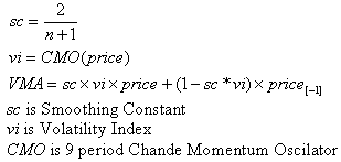
Variable Moving Average: A Variable Moving Average is an exponential moving average that automatically adjusts the smoothing weight based on the volatility of the data series. The more volatile the data is, the more weight is given to the more recent values. The Variable Moving Average solves a problem with most moving averages. In times of low volatility, such as when the price is trending, the moving average time period should be shorter to be sensitive to the inevitable break in the trend. Whereas, in more volatile non-trending times, the moving average time period should be longer to filter out the choppiness. Almost any measure of volatility can be used in calculating the Variable Moving Average, however, most implementations use a 9 period Chande Momentum Oscillator (CMO). The Variable Moving Average is also known as the VIDYA Indicator. The Variable Moving Average was developed by Tushar S. Chande and first presented in his March, 1992 article in Technical Analysis of Stocks & Commodities magazine, in which a standard deviation was used as the Volatility Index. In his October, 1995 article in the same magazine, Chande modified the VIDYA to use his own Chande Momentum Oscillator (CMO) as the Volatility Index. See also Exponential MA, Least Squares MA, Simple MA, Triangular MA, Weighted MA, Welles MA, Volume Adjusted MA, Zero Lag Exponential MA, DEMA, TEMA and T3.
Formula:
Vertical Horizontal Filter (VHF): The Vertical Horizontal Filter (VHF) determines whether prices are trending. When the VHF is rising, it indicates the formation of a trend. Higher VHF values indicate a stronger trend. When the VHF is falling, it indicates the trend is ending and price is becoming congested. Very low VHF values indicate a trend may follow. The Vertical Horizontal Filter was developed by Adam White.
Formula:
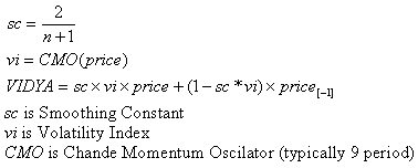
VIDYA: VIDYA is an acronym of Variable Index DYnamic Average. The VIDYA is an exponential moving average that automatically adjusts the smoothing weight based on the volatility of the data series. The more volatile the data is, the more weight is given to the more recent values. The VIDYA solves a problem with most moving averages. In times of low volatility, such as when the price is trending, the moving average time period should be shorter to be sensitive to the inevitable break in the trend. Whereas, in more volatile non-trending times, the moving average time period should be longer to filter out the choppiness. The VIDYA is also known as the Variable Moving Average. The VIDYA was developed by Tushar S. Chande and first presented in his March, 1992 article in Technical Analysis of Stocks & Commodities magazine, in which a standard deviation was used as the Volatility Index. In his October, 1995 article in the same magazine, Chande modified the VIDYA to use his own Chande Momentum Oscillator (CMO) as the Volatility Index.
Formula:
Volume Adjusted Moving Average: The Volume Weighted Moving Average is a weighted moving average that uses the volume as the weighting factor, so that higher volume days have more weight. It is a non-cumulative moving average, in that only data within the time period is used in the calculation. See also Exponential MA, Least Squares MA, Simple MA, Triangular MA, Weighted MA, Welles MA, Variable MA, Zero Lag Exponential MA, DEMA, TEMA and T3.
Formula:
Weighted Close: The Weighted Close is the average of the high, low and close of a bar, but the close is weighted, actually counted twice. It is used in the calculation of several indicators. It can be used to smooth an indicator that normally takes just the closing price as input. See also Average Price, Median Price and Typical Price.
Formula:
Weighted Moving Average: The Weighted Moving Average calculates a weight for each value in the series. The more recent values are assigned greater weights. The Weighted Moving Average is similar to a Simple Moving average in that it is not cumulative, that is, it only includes values in the time period (unlike an Exponential Moving Average). The Weighted Moving Average is similar to an Exponential Moving Average in that more recent data has a greater contribution to the average. See also Exponential MA, Least Squares MA, Simple MA, Triangular MA, Welles MA, Variable MA, Volume Adjusted MA, Zero Lag Exponential MA, DEMA, TEMA and T3.
Formula:
Welles Wilder Moving Average: The Welles Wilder method of calculating moving averages is very similar to a Simple Moving Average. Both calculations provide similar results. Welles designed his formula to be easily computed by hand or with a simple calculator. For the sake of consistency Welles\' Moving Averages are used in all Welles indicator formulas (ADX, ADXR and ATR). See also Exponential MA, Least Squares MA, Simple MA, Triangular MA, Weighted MA, Variable MA, Volume Adjusted MA, Zero Lag Exponential MA, DEMA, TEMA and T3.
Formula:
Welles Wilder Summation: The Welles Sum is the Welles Wilder method of creating the moving sum of a data series. Each value is the sum of the last n periods. Welles designed his formula to be easily computed by hand or with a simple calculator. The numbers will vary slightly from a simple (arithmetic) sum. For consistency with the original formulas, the Welles Sum is used in the calculation of Welles Wilder\'s indicators (the +/-DI and by extension the DX, ADX, ADXR). See also Moving Sum.
Formula:
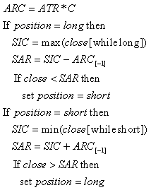
Welles Wilder Volatility System: This function calculates the componants of the Welles Wilder Volatility System. The components are as follows: ARC - the Average True Range (ATR) times a constant.\r\nSIC - SIgnificant Close, the extreme favorable close price reached while in the trade.\r\nStop And Reverse point, a point defined by the distance between the ARC and SIC. The point at which a trade should be made close the current position and open a new position in the opposite direction. This occurs when the price breaks above/below the SAR. The Volatility System was developed by J. Welles Wilder and is described in his 1978 book New Concepts In Technical Trading Systems.
Formula:
Williams Accumulation/Distribution: Williams Accumulation/Distribution indicator measures market pressure. Look for divergence with price. When the price makes a new low, but the AD does not, look for the price to turn up, and vice versa. The Williams Accumulation/Distribution Indicator is also know as the Williams AD. It was developed by Larry Williams.
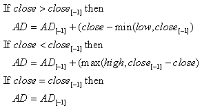
Formula:
Williams %R: The Williams %R is similar to an unsmoothed Stochastic %K. The values range from zero to 100, and are charted on an inverted scale, that is, with zero at the top and 100 at the bottom. Values below 20 indicate an overbought condition and a sell signal is generated when it crosses the 20 line. Values over 80 indicate an oversold condition and a buy signal is generated when it crosses the 80 line. The %R indicator was developed by Larry Williams.
Formula:
Zero Lag Exponential Moving Average: The Zero-Lag Exponential Moving Average is a variation on the Exponential Moving Average. The Zero-Lag keeps the benefit of the heavier weighting of recent values, but attempts to remove lag by subtracting older data to minimize the cumulative effect. See also Exponential MA, Least Squares MA, Simple MA, Triangular MA, Weighted MA, Welles MA, Variable MA, Volume Adjusted MA, DEMA, TEMA and T3.
Formula:
Zig Zag: The Zig Zag filters out small movements in price to highlight trends. It looks for price moves greater than the threshold level and plots straight lines between those points. The Zig Zag is more of a visual tool than an indicator. It is non-predictive, in fact, the formula looks forward in time to find the zig zag points. The purpose of the Zig Zag is to make chart patterns clearer.
Spread: The Spread is the difference between two prices series. You can also apply a Spread to other different indicators applied to a chart, such as a Moving Average.